%load_ext autoreload
%autoreload 2
from pathlib import Path
from typing import Literal

from matplotlib import pyplot as plt
from shapely.geometry import Point
from scipy.interpolate import interp1d
from scipy.signal import find_peaks
import numpy as np

from s2shores.bathy_debug.spatial_dft_bathy_estimator_debug import SpatialDFTBathyEstimatorDebug

from s2shores.bathy_physics import celerity_offshore, period_offshore, wavelength_offshore
from s2shores.generic_utils.image_filters import circular_masking
from s2shores.generic_utils.image_utils import normalized_cross_correlation
from s2shores.generic_utils.signal_utils import find_period_from_zeros
from s2shores.generic_utils.symmetric_radon import symmetric_radon
from s2shores.image_processing.waves_radon import linear_directions
from s2shores.bathy_debug.display_utils import get_display_title_with_kernel
from s2shores.bathy_debug.sinogram_display import (
    build_sinogram_display,
    build_sinogram_difference_display,
    build_sinogram_1D_display_master,
    build_sinogram_1D_cross_correlation,
    build_sinogram_1D_display_slave,
    build_sinogram_2D_cross_correlation,
)
from s2shores.bathy_debug.spatial_dft_wave_fields_display import build_dft_sinograms_spectral_analysis
from s2shores.bathy_debug.sinogram_display import (
    build_sinogram_display,
    build_sinogram_difference_display,
    build_sinogram_spectral_display,
    build_correl_spectrum_matrix)

from s2shores.bathy_debug.spatial_dft_wave_fields_display import build_dft_sinograms
from s2shores.global_bathymetry.bathy_config import (
    BathyConfig,
    GlobalEstimatorConfig,
    SpatialDFTConfig,
)
from s2shores.waves_exceptions import WavesEstimationError, NotExploitableSinogram
from utils import initialize_sequential_run, read_config, plot_waves_row, build_ortho_sequence
---------------------------------------------------------------------------
ModuleNotFoundError                       Traceback (most recent call last)
Cell In[2], line 4
      1 from pathlib import Path
      2 from typing import Literal
----> 4 from matplotlib import pyplot as plt
      5 from shapely.geometry import Point
      6 from scipy.interpolate import interp1d

ModuleNotFoundError: No module named 'matplotlib'
In case of a specfic server setup, specify the paths for
- os.environ["PROJ_DATA"]
- os.environ["GDAL_DATA"]
- os.environ["GDAL_DRIVER_PATH"]
- os.environ["CONDA_PREFIX"]
"""
import os
os.environ["PROJ_DATA"]="..../share/proj"
os.environ["GDAL_DATA"]="..../share/gdal"
os.environ["GDAL_DRIVER_PATH"]="..../lib/gdalplugins"
os.environ["CONDA_PREFIX"]="..../s2shores"
"""
Coastal Bathymetry Estimation via Spatial DFT
This notebook implements a bathymetric method using satellite imagery based on spatial DFT and the linear relationship between water depth and wave kinematics.
Wave kinematics are inferred through the spatial DFT of the wave field, measured from two satellite images acquired within a short time interval.
By leveraging the theory of linear wave dispersion in shallow water, bathymetry can be estimated from the wavelength of the waves.
Notebook Objective
This notebook provides an experimental and interactive environment to:
explore and adjust the key processing steps,
quickly test different parameters and method variations,
support iterative development of the processing workflow in a prototyping context.
Notebook Summary
Preprocess the images: Apply filters on the images.
Compute the Radon transforms: Compute Radon transforms on all images.
Find the directions: Calculate the propagation directions of the waves.
Prepare refinement: Filter out and group found directions together.
Find spectral peaks: Compute the interpolated DFTs in each of the filtered directions and find the peaks.
base_path = Path("../tests/data/products").resolve()
test_case: Literal["7_4", "8_2"] = "8_2"
method: Literal["spatial_corr", "spatial_dft", "temporal_corr"] = "spatial_dft"

product_path: Path = base_path / "products" / f"SWASH_{test_case}/testcase_{test_case}.tif"
config_path: Path = base_path / f"reference_results/debug_pointswash_{method}/wave_bathy_inversion_config.yaml"
debug_file: Path = base_path / f"debug_points/debug_points_SWASH_{test_case}.yaml"
# config = read_config(config_path=config_path)

# OR

config = BathyConfig(
    GLOBAL_ESTIMATOR=GlobalEstimatorConfig(
        WAVE_EST_METHOD="SPATIAL_DFT",
        SELECTED_FRAMES=[10, 13],
        DXP=50,
        DYP=500,
        NKEEP=5,
        WINDOW=400,
        SM_LENGTH=100,
        MIN_D=2,
        MIN_T=3,
        MIN_WAVES_LINEARITY=0.01,
    ),
    SPATIAL_DFT=SpatialDFTConfig(
        PROMINENCE_MAX_PEAK=0.3,
        PROMINENCE_MULTIPLE_PEAKS=0.1,
        UNWRAP_PHASE_SHIFT=False,
        ANGLE_AROUND_PEAK_DIR=10,
        STEP_T=0.05,
    )
)
If you want to change any parameter of the configuration, modify the values of the object config by overriding the values of the attributes.
Example:
config.parameter = "new_value"
bathy_estimator, ortho_bathy_estimator = initialize_sequential_run(
    product_path=product_path,
    config=config,
    delta_time_provider=None,
)

plt_min = bathy_estimator.local_estimator_params['DEBUG']['PLOT_MIN']
plt_max = bathy_estimator.local_estimator_params['DEBUG']['PLOT_MAX']
/home/geoffrey/miniconda3/envs/s2shores_env/lib/python3.12/site-packages/distributed/node.py:187: UserWarning: Port 8787 is already in use.
Perhaps you already have a cluster running?
Hosting the HTTP server on port 39321 instead
  warnings.warn(
/home/geoffrey/miniconda3/envs/s2shores_env/lib/python3.12/site-packages/osgeo/gdal.py:312: FutureWarning: Neither gdal.UseExceptions() nor gdal.DontUseExceptions() has been explicitly called. In GDAL 4.0, exceptions will be enabled by default.
  warnings.warn(
estimation_point = Point(451.0, 499.0)
ortho_sequence = build_ortho_sequence(ortho_bathy_estimator, estimation_point)

selected_directions = linear_directions(
    angle_min=min(-180, plt_min),
    angle_max=max(180, plt_max),
    angles_step=1,
)

local_estimator = SpatialDFTBathyEstimatorDebug(
    estimation_point,
    ortho_sequence,
    bathy_estimator,
    selected_directions,
)

if not local_estimator.can_estimate_bathy():
    raise WavesEstimationError("Cannot estimate bathy.")
Preprocess images
Modified attributes:
local_estimator.ortho_sequence.<elements>.pixels
from s2shores.generic_utils.image_filters import desmooth, detrend

def custom_filter(img, param1, param2):
    """My custom filter."""
    return img


if False:
    local_estimator.preprocess_images()
else:
    preprocessing_filters = [(detrend, [])]

    if bathy_estimator.smoothing_requested:
        # FIXME: pixels necessary for smoothing are not taken into account, thus
        # zeros are introduced at the borders of the window.

        preprocessing_filters += [
            (desmooth,
             [bathy_estimator.smoothing_lines_size,
              bathy_estimator.smoothing_columns_size]),
            # Remove tendency possibly introduced by smoothing, specially on the shore line
            (detrend, []),
            # Add your custom filters here
            # Ex: (custom_filter, [param1, param2])
        ]


    for image in local_estimator.ortho_sequence:
        filtered_image = image.apply_filters(preprocessing_filters)
        image.pixels = filtered_image.pixels
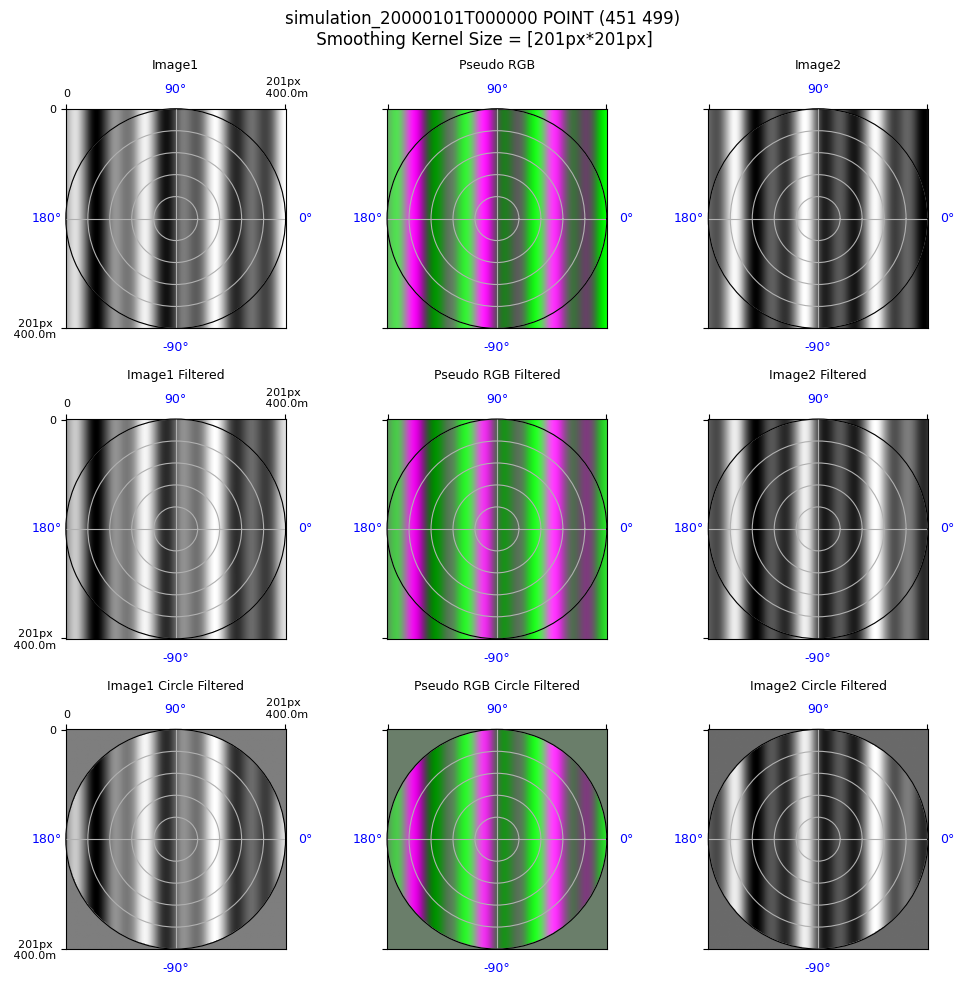
Display processed images
if False:
    build_waves_images_spatial_correl(local_estimator)
else:
    nrows = 3
    ncols = 3
    fig, axs = plt.subplots(nrows=nrows, ncols=ncols, figsize=(10, 10))
    fig.suptitle(get_display_title_with_kernel(local_estimator), fontsize=12)

    first_image = local_estimator.ortho_sequence[0]
    second_image = local_estimator.ortho_sequence[1]

    # First Plot line = Image1 / pseudoRGB / Image2
    plot_waves_row(fig=fig,
                   axs=axs,
                   row_number=0,
                   pixels1=first_image.original_pixels,
                   resolution1=first_image.resolution,
                   pixels2=second_image.original_pixels,
                   resolution2=first_image.resolution,
                   nrows=3,
                   ncols=3)
    # Second Plot line = Image1 Filtered / pseudoRGB Filtered/ Image2 Filtered
    plot_waves_row(fig=fig,
                   axs=axs,
                   row_number=1,
                   pixels1=first_image.pixels,
                   resolution1=first_image.resolution,
                   pixels2=second_image.pixels,
                   resolution2=first_image.resolution,
                   title_suffix=" Filtered",
                   nrows=3,
                   ncols=3)

    # Third Plot line = Image1 Circle Filtered / pseudoRGB Circle Filtered/ Image2 Circle Filtered
    plot_waves_row(fig=fig,
                   axs=axs,
                   row_number=2,
                   pixels1=first_image.pixels * first_image.circle_image,
                   resolution1=first_image.resolution,
                   pixels2=second_image.pixels * second_image.circle_image,
                   resolution2=first_image.resolution,
                   title_suffix=" Circle Filtered",
                   nrows=3,
                   ncols=3)
    plt.tight_layout()
Compute radon transforms
New elements:
local_estimator.radon_transforms
# Reset radon transforms when cell is re-run
local_estimator.radon_transforms = []
sampling_frequencies = []

if False:
    local_estimator.compute_radon_transforms()
    sampling_frequencies = [
        radon_transform.sampling_frequency
        for radon_transform in local_estimator.radon_transforms
    ]
else:
    for image in local_estimator.ortho_sequence:
        sampling_frequencies.append(1. / image.resolution)

        pixels = circular_masking(image.pixels.copy())
        radon_transform = symmetric_radon(image=pixels, theta=selected_directions)

        local_estimator.radon_transforms.append({
            direction: radon_transform[:, idx]
            for idx, direction in enumerate(selected_directions)
        })
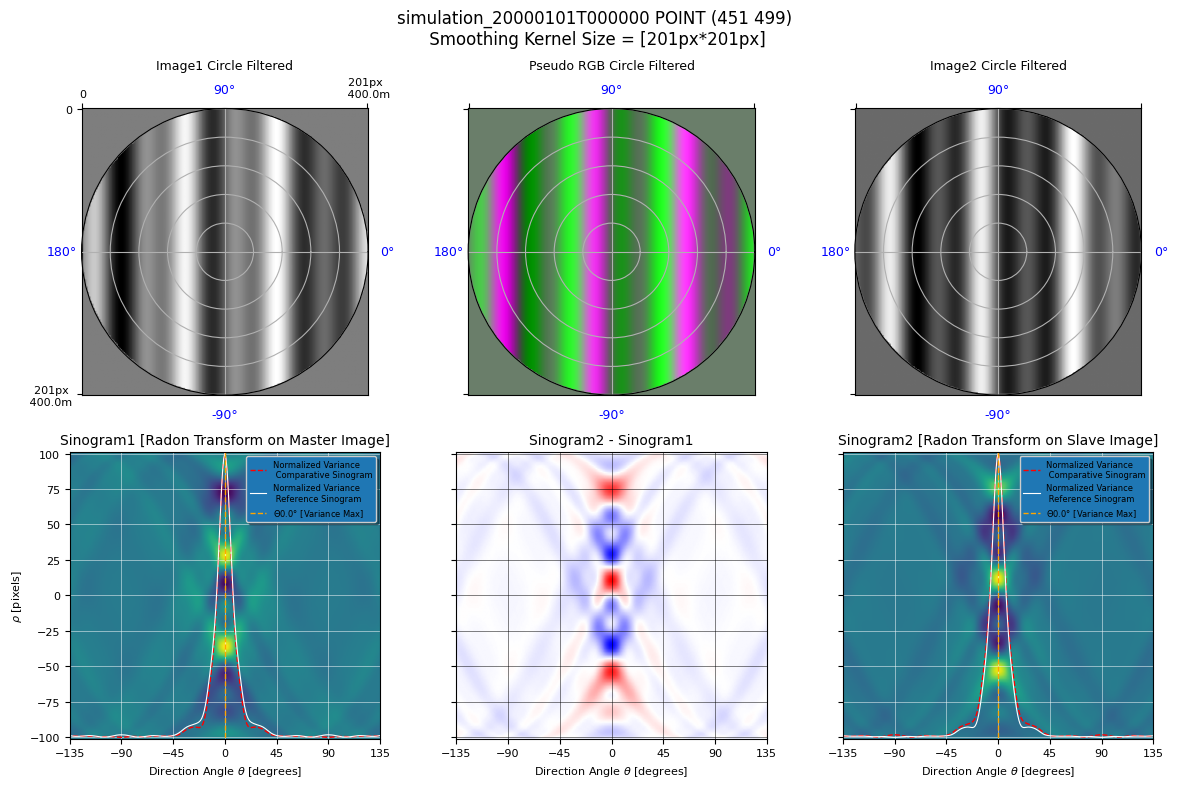
Plot sinograms
if False:
    # Use this when computing radon transforms with the standard method
    build_dft_sinograms(local_estimator)
else:
    nrows = 2
    ncols = 3
    fig, axs = plt.subplots(nrows=nrows, ncols=ncols, figsize=(12, 8))
    fig.suptitle(get_display_title_with_kernel(local_estimator), fontsize=12)
    first_image = local_estimator.ortho_sequence[0]
    second_image = local_estimator.ortho_sequence[1]

    # First Plot line = Image1 Circle Filtered / pseudoRGB Circle Filtered/ Image2 Circle Filtered
    plot_waves_row(
        fig=fig,
        axs=axs,
        row_number=0,
        pixels1=first_image.pixels * first_image.circle_image,
        resolution1=first_image.resolution,
        pixels2=second_image.pixels * second_image.circle_image,
        resolution2=first_image.resolution,
        nrows=nrows,
        ncols=ncols,
        title_suffix=" Circle Filtered",
    )

    # Second Plot line = Sinogram1 / Sinogram2-Sinogram1 / Sinogram2
    first_radon_transform = local_estimator.radon_transforms[0]
    second_radon_transform = local_estimator.radon_transforms[1]


    first_iter = next(iter(first_radon_transform.values()))
    nb_samples = first_iter.shape[0]

    sinogram1 = np.empty((nb_samples, len(selected_directions)))
    sinogram2 = np.empty((nb_samples, len(selected_directions)))

    for index, direction in enumerate(selected_directions):
        sinogram1[:, index] = first_radon_transform[direction]
        sinogram2[:, index] = second_radon_transform[direction]

    radon_difference = (
        (sinogram2 / np.abs(sinogram2).max())
        - (sinogram1 / np.abs(sinogram1).max())
    )

    build_sinogram_display(
        axes=axs[1, 0],
        title='Sinogram1 [Radon Transform on Master Image]',
        values1=sinogram1,
        directions=selected_directions,
        values2=sinogram2,
        plt_min=plt_min,
        plt_max=plt_max,
    )
    build_sinogram_difference_display(
        axes=axs[1, 1],
        title='Sinogram2 - Sinogram1',
        values=radon_difference,
        directions=selected_directions,
        plt_min=plt_min,
        plt_max=plt_max,
        cmap='bwr',
    )
    build_sinogram_display(
        axes=axs[1, 2],
        title='Sinogram2 [Radon Transform on Slave Image]',
        values1=sinogram2,
        directions=selected_directions,
        values2=sinogram1,
        plt_min=plt_min,
        plt_max=plt_max,
        ordonate=False,
    )

    plt.tight_layout()
Find directions
New variables:
peaks
New attributes:
- local_estimator.metrics['standard_dft']
def dft(values: np.ndarray):
    dft_frequencies = np.fft.fftfreq(values.size)[0:int(np.ceil(values.size / 2))]
    return np.fft.fft(values)[0:dft_frequencies.size]

def get_sinograms_standard_dfts(radon_transform: dict[float, np.ndarray], directions_range: np.ndarray | list = None):
    if directions_range is None:
        directions_range = list(radon_transform.keys())

    fft_sino_length = dft(radon_transform[directions_range[0]]).size
    result = np.empty((fft_sino_length, len(directions_range)), dtype=np.complex128)
    for result_index, direction in enumerate(directions_range):
        sinogram = radon_transform[direction]
        result[:, result_index] = dft(sinogram)
    return result


if False:
    peaks = local_estimator.find_directions()
else:
    # TODO: modify directions finding such that only one radon transform is computed (50% gain)
    sino1_fft = get_sinograms_standard_dfts(local_estimator.radon_transforms[0])
    sino2_fft = get_sinograms_standard_dfts(local_estimator.radon_transforms[1])

    sinograms_correlation_fft = sino1_fft * np.conj(sino2_fft)
    phase_shift = np.angle(sinograms_correlation_fft)
    spectrum_amplitude = np.abs(sinograms_correlation_fft)
    total_spectrum = np.abs(phase_shift) * spectrum_amplitude

    max_heta = np.max(total_spectrum, axis=0)
    total_spectrum_normalized = max_heta / np.max(max_heta)

    # TODO: possibly apply symmetry to totalSpecMax_ref in find directions
    peaks, values = find_peaks(total_spectrum_normalized,
                               prominence=local_estimator.local_estimator_params['PROMINENCE_MAX_PEAK'])
    prominences = values['prominences']

    # Start: local_estimator._process_peaks(peaks, prominences)
    print('initial peaks: ', peaks)
    peaks_pairs = []
    for index1 in range(peaks.size - 1):
        for index2 in range(index1 + 1, peaks.size):
            if abs(peaks[index1] - peaks[index2]) == 180:
                peaks_pairs.append((index1, index2))
                break

    print('peaks_pairs: ', peaks_pairs)

    filtered_peaks_dir = []
    # Keep only one direction from each pair, with the greatest prominence
    for index1, index2 in peaks_pairs:
        if abs(prominences[index1] - prominences[index2]) < 100:
            # Prominences almost the same, keep lowest index
            filtered_peaks_dir.append(peaks[index1])
        else:
            if prominences[index1] > prominences[index2]:
                filtered_peaks_dir.append(peaks[index1])
            else:
                filtered_peaks_dir.append(peaks[index2])

    print('peaks kept from peaks_pairs: ', filtered_peaks_dir)

    # Add peaks which do not belong to a pair
    for index in range(peaks.size):
        found_in_pair = False
        for index1, index2 in peaks_pairs:
            if index in (index1, index2):
                found_in_pair = True
                break
        if not found_in_pair:
            filtered_peaks_dir.append(peaks[index])

    print('final peaks after adding isolated peaks: ', sorted(filtered_peaks_dir))
    peaks = np.array(sorted(filtered_peaks_dir))

    if peaks.size == 0:
        raise WavesEstimationError('Unable to find any directional peak')

    local_estimator.metrics['standard_dft'] = {
        'sinograms_correlation_fft': sinograms_correlation_fft,
        'total_spectrum': total_spectrum,
        'max_heta': max_heta,
        'total_spectrum_normalized': total_spectrum_normalized,
    }
initial peaks:  [180]
peaks_pairs:  []
peaks kept from peaks_pairs:  []
final peaks after adding isolated peaks:  [180]
Prepare refinement
New variables:
directions
if False:
    directions = local_estimator.prepare_refinement(peaks)
else:
    directions = []
    if peaks.size > 0:
        for peak_index in range(0, peaks.size):
            angles_half_range = local_estimator.local_estimator_params['ANGLE_AROUND_PEAK_DIR']
            direction_index = peaks[peak_index]
            tmp = np.arange(
                max(direction_index - angles_half_range, 0),
                min(direction_index + angles_half_range + 1, 360),
                dtype=np.int64,
            )
            directions_range = np.array(sorted(local_estimator.radon_transforms[0].keys()))[tmp]
            directions.append(directions_range)
Find spectral peaks
New attributes:
- local_estimator.metrics['kfft']
- local_estimator.metrics['totSpec']
- local_estimator.metrics['interpolated_dft']
Modified attributes:
local_estimator.bathymetry_estimations
from s2shores.image_processing.waves_sinogram import WavesSinogram

def get_sinograms_interpolated_dfts(sinograms, wavenumbers, sampling_frequency, directions = None):
    if wavenumbers.size == 0:
        raise ValueError('DFT interpolation requires at least 1 frequency')

    directions = sinograms.keys() if directions is None else directions
    normalized_frequencies = wavenumbers / sampling_frequency

    fft_sino_length = interpolate_dft(sinograms[next(iter(directions))], normalized_frequencies).size
    interpolated_dfts = np.empty((fft_sino_length, len(directions)), dtype=np.complex128)
    for result_index, direction in enumerate(directions):
        interpolated_dfts[:, result_index] = interpolate_dft(sinograms[direction], normalized_frequencies)

    return interpolated_dfts, normalized_frequencies


def interpolate_dft(sinogram, frequencies):
    if isinstance(sinogram, WavesSinogram):
        sinogram = sinogram.values
    unity_roots = get_unity_roots(frequencies, sinogram.size)
    return np.dot(unity_roots, sinogram)


def get_unity_roots(frequencies: np.ndarray, number_of_roots: int) -> np.ndarray:
    roots_indexes = np.arange(number_of_roots)
    working_frequencies = np.expand_dims(frequencies, axis=1)
    return np.exp(-2j * np.pi * working_frequencies * roots_indexes)

# Reset for re-runs
local_estimator.bathymetry_estimations.clear()

if False:
    local_estimator.find_spectral_peaks(directions)
else:
    wavenumbers = local_estimator.full_linear_wavenumbers
    sino_ffts: list[tuple[np.ndarray, np.ndarray]] = []

    for directions_range in directions:
        # Detailed analysis of the signal for positive phase shifts
        sino1_fft, dft_frequencies1 = get_sinograms_interpolated_dfts(
            local_estimator.radon_transforms[0],
            wavenumbers,
            sampling_frequencies[0],
            directions_range)
        sino2_fft, dft_frequencies2 = get_sinograms_interpolated_dfts(
            local_estimator.radon_transforms[1],
            wavenumbers,
            sampling_frequencies[1],
            directions_range)


        phase_shift, spectrum_amplitude, sinograms_correlation_fft = \
            local_estimator._cross_correl_spectrum(sino1_fft, sino2_fft)
        total_spectrum = np.abs(phase_shift) * spectrum_amplitude
        max_heta = np.max(total_spectrum, axis=0)
        total_spectrum_normalized = max_heta / np.max(max_heta)

        peaks_freq = find_peaks(total_spectrum_normalized,
                                prominence=local_estimator.local_estimator_params['PROMINENCE_MULTIPLE_PEAKS'])
        peaks_freq = peaks_freq[0]
        peaks_wavenumbers_ind = np.argmax(total_spectrum[:, peaks_freq], axis=0)


        for index, direction_index in enumerate(peaks_freq):
            estimated_direction = directions_range[direction_index]
            wavenumber_index = peaks_wavenumbers_ind[index]
            estimated_phase_shift = phase_shift[wavenumber_index, direction_index]

            peak_sinogram = local_estimator.radon_transforms[0][estimated_direction]
            normalized_frequency = dft_frequencies1[wavenumber_index]
            wavenumber = normalized_frequency * sampling_frequencies[0]

            energy = total_spectrum[wavenumber_index, direction_index]
            estimation = local_estimator.save_wave_field_estimation(estimated_direction, wavenumber,
                                                         estimated_phase_shift, energy)
            local_estimator.bathymetry_estimations.append(estimation)


        local_estimator.metrics['kfft'] = wavenumbers
        local_estimator.metrics['totSpec'] = np.abs(total_spectrum) / np.mean(total_spectrum)
        local_estimator.metrics['interpolated_dft'] = {
            'max_heta': max_heta,
            'total_spectrum_normalized': total_spectrum_normalized,
            'sinograms_correlation_fft': sinograms_correlation_fft,
            'total_spectrum': total_spectrum,
            'phase_shift': phase_shift,
            'directions': directions_range,
        }


for estimations in local_estimator.bathymetry_estimations:
    print(estimations)
Geometry:   direction: 0.0° wavelength: 136.08 (m) wavenumber: 0.007349 (m-1)
Dynamics:   period:  9.21 (s)  celerity: 14.78 (m/s)
Wave Field Estimation:
  delta time: 3.000 (s) stroboscopic factor: 0.326 (unitless)
  delta position: 44.34 (m)  delta phase:  2.05 (rd)
Bathymetry inversion: depth:   inf (m)  gamma: 1.031  offshore period:  9.35 (s)  shallow water period: 30.77 (s)  relative period:  1.02  relative wavelength:  0.97  gravity: 9.780 (s)
Bathymetry Estimation:  stroboscopic factor low depth: 0.098  stroboscopic factor offshore: 0.321
    energy: 423803640.35 (???)  energy ratio: 437043740.55
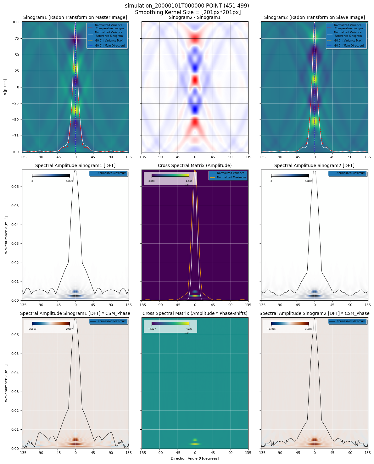
Display spectral analysis
if False:
    build_dft_sinograms_spectral_analysis(local_estimator)
else:
    nrows = 3
    ncols = 3
    fig, axs = plt.subplots(nrows=nrows, ncols=ncols, figsize=(12, 15))
    fig.suptitle(get_display_title_with_kernel(local_estimator), fontsize=12)


    first_radon_transform = local_estimator.radon_transforms[0]
    second_radon_transform = local_estimator.radon_transforms[1]

    # First Plot line = Sinogram1 / Sinogram2-Sinogram1 / Sinogram2
    sinogram1 = np.empty((nb_samples, len(selected_directions)))
    sinogram2 = np.empty((nb_samples, len(selected_directions)))
    directions1 = selected_directions
    directions2 = selected_directions

    for index, direction in enumerate(selected_directions):
        sinogram1[:, index] = first_radon_transform[direction]
        sinogram2[:, index] = second_radon_transform[direction]

    radon_difference = (sinogram2 / np.max(np.abs(sinogram2))) - \
        (sinogram1 / np.max(np.abs(sinogram1)))

    # get main direction
    estimations = local_estimator.bathymetry_estimations
    sorted_estimations_args = estimations.argsort_on_attribute(
        local_estimator.final_estimations_sorting)
    main_direction = estimations.get_estimations_attribute('direction')[
        sorted_estimations_args[0]]

    build_sinogram_display(
        axs[0, 0], 'Sinogram1 [Radon Transform on Master Image]',
        sinogram1, selected_directions, sinogram2, plt_min, plt_max, main_direction, abscissa=False)
    build_sinogram_difference_display(
        axs[0, 1], 'Sinogram2 - Sinogram1', radon_difference, selected_directions, plt_min, plt_max,
        abscissa=False, cmap='bwr')
    build_sinogram_display(
        axs[0, 2], 'Sinogram2 [Radon Transform on Slave Image]', sinogram2, selected_directions, sinogram1,
        plt_min, plt_max, main_direction, ordonate=False, abscissa=False)


    # Second Plot line = Spectral Amplitude of Sinogram1 [after DFT] / CSM Amplitude /
    # Spectral Amplitude of Sinogram2 [after DFT]
    sino1_fft = get_sinograms_standard_dfts(first_radon_transform, selected_directions)
    sino2_fft = get_sinograms_standard_dfts(second_radon_transform, selected_directions)
    kfft = local_estimator._metrics['kfft']
    csm_phase, _, _ = local_estimator._cross_correl_spectrum(sino1_fft, sino2_fft)

    build_sinogram_spectral_display(
        axs[1, 0],
        'Spectral Amplitude Sinogram1 [DFT]',
        np.abs(sino1_fft),
        directions1,
        kfft,
        plt_min,
        plt_max,
        abscissa=False,
        cmap='cmc.oslo_r')
    build_correl_spectrum_matrix(
        axs[1, 1],
        local_estimator,
        sino1_fft,
        sino2_fft,
        kfft,
        plt_min,
        plt_max,
        'amplitude',
        'Cross Spectral Matrix (Amplitude)',
        directions=directions1)
    build_sinogram_spectral_display(
        axs[1, 2],
        'Spectral Amplitude Sinogram2 [DFT]',
        np.abs(sino2_fft),
        directions2,
        kfft,
        plt_min,
        plt_max,
        ordonate=False,
        abscissa=False,
        cmap='cmc.oslo_r')

    # Third Plot line = Spectral Amplitude of Sinogram1 [after DFT] * CSM Phase /
    # CSM Amplitude * CSM Phase / Spectral Amplitude of Sinogram2 [after DFT] * CSM Phase

    build_sinogram_spectral_display(
        axs[2, 0],
        'Spectral Amplitude Sinogram1 [DFT] * CSM_Phase',
        np.abs(sino1_fft) * csm_phase,
        selected_directions,
        kfft,
        plt_min,
        plt_max,
        abscissa=False,
        cmap='cmc.vik')
    build_correl_spectrum_matrix(
        axs[2, 1],
        local_estimator,
        sino1_fft,
        sino2_fft,
        kfft,
        plt_min,
        plt_max,
        'phase',
        'Cross Spectral Matrix (Amplitude * Phase-shifts)',
        directions=directions1)
    build_sinogram_spectral_display(
        axs[2, 2],
        'Spectral Amplitude Sinogram2 [DFT] * CSM_Phase',
        np.abs(sino2_fft) * csm_phase,
        selected_directions,
        kfft,
        plt_min,
        plt_max,
        ordonate=False,
        abscissa=False,
        cmap='cmc.vik')
    plt.tight_layout()
/tmp/ipykernel_31300/682541998.py:119: UserWarning: This figure includes Axes that are not compatible with tight_layout, so results might be incorrect.
  plt.tight_layout()
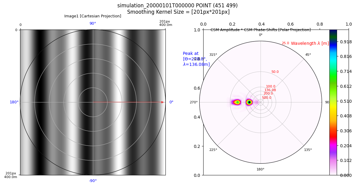
Display polar image
from s2shores.bathy_debug.spatial_dft_wave_fields_display import build_polar_images_dft
from s2shores.bathy_debug.waves_image_display import build_display_waves_image
from s2shores.bathy_debug.polar_display import build_polar_display

if False:
    build_polar_images_dft(local_estimator)
else:
    nrows = 1
    ncols = 2
    fig, axs = plt.subplots(nrows=nrows, ncols=ncols, figsize=(12, 6))
    fig.suptitle(get_display_title_with_kernel(local_estimator), fontsize=12)

    estimations = local_estimator.bathymetry_estimations
    best_estimation_idx = estimations.argsort_on_attribute(
        local_estimator.final_estimations_sorting)[0]
    main_direction = estimations.get_estimations_attribute('direction')[best_estimation_idx]
    ener_max = estimations.get_estimations_attribute('energy_ratio')[best_estimation_idx]
    main_wavelength = estimations.get_estimations_attribute('wavelength')[best_estimation_idx]
    dir_max_from_north = (270 - main_direction) % 360
    arrows = [(wfe.direction, wfe.energy_ratio) for wfe in estimations]

    print('ARROWS', arrows)
    first_image = local_estimator.ortho_sequence[0]

    # First Plot line = Image1 / pseudoRGB / Image2
    build_display_waves_image(
        fig,
        axs[0],
        'Image1 [Cartesian Projection]',
        first_image.original_pixels,
        resolution=first_image.resolution,
        subplot_pos=[nrows, ncols, 1],
        directions=arrows,
        cmap='gray')

    csm_phase, spectrum_amplitude, sinograms_correlation_fft = \
        local_estimator._cross_correl_spectrum(sino1_fft, sino2_fft)
    csm_amplitude = np.abs(sinograms_correlation_fft)

    # Retrieve arguments corresponding to the arrow with the maximum energy
    arrow_max = (dir_max_from_north, ener_max, main_wavelength)

    print('-->ARROW SIGNING THE MAX ENERGY [DFN, ENERGY, WAVELENGTH]]=', arrow_max)
    polar = csm_amplitude * csm_phase

    # set negative values to 0 to avoid mirror display
    polar[polar < 0] = 0
    build_polar_display(
        fig,
        axs[1],
        'CSM Amplitude * CSM Phase-Shifts [Polar Projection]',
        local_estimator,
        polar,
        first_image.resolution,
        dir_max_from_north,
        main_wavelength,
        subplot_pos=[1, 2, 2],
        directions=selected_directions,
        nb_wavenumbers=sinogram1.shape[0])
    plt.tight_layout()
ARROWS [(0.0, 437043740.5502732)]
-->ARROW SIGNING THE MAX ENERGY [DFN, ENERGY, WAVELENGTH]]= (270.0, 437043740.5502732, 136.07621106623083)
MAIN DIRECTION 0.0
DIRECTION FROM NORTH 270.0
DELTA TIME 3.0
DELTA PHASE 2.047244075785284