%load_ext autoreload
%autoreload 2

The autoreload extension is already loaded. To reload it, use:
  %reload_ext autoreload

from pathlib import Path
from typing import Literal

from matplotlib import pyplot as plt
from shapely.geometry import Point
from scipy.interpolate import interp1d
from scipy.signal import find_peaks
import numpy as np

from s2shores.bathy_debug.spatial_correlation_bathy_estimator_debug import SpatialCorrelationBathyEstimatorDebug
from s2shores.bathy_debug.spatial_correlation_wave_fields_display import (
    build_sinograms_spatial_correlation,
    build_waves_images_spatial_correl,
)

from s2shores.bathy_physics import celerity_offshore, period_offshore, wavelength_offshore
from s2shores.generic_utils.image_filters import circular_masking
from s2shores.generic_utils.image_utils import normalized_cross_correlation
from s2shores.generic_utils.signal_utils import find_period_from_zeros
from s2shores.generic_utils.symmetric_radon import symmetric_radon
from s2shores.bathy_debug.display_utils import get_display_title_with_kernel
from s2shores.bathy_debug.sinogram_display import (
    build_sinogram_display,
    build_sinogram_difference_display,
    build_sinogram_1D_display_master,
    build_sinogram_1D_cross_correlation,
    build_sinogram_1D_display_slave,
    build_sinogram_2D_cross_correlation,
)
from s2shores.global_bathymetry.bathy_config import (
    BathyConfig,
    GlobalEstimatorConfig,
    SpatialCorrelationConfig,
)
from s2shores.waves_exceptions import WavesEstimationError, NotExploitableSinogram
from utils import (
    initialize_sequential_run,
    read_config,
    plot_waves_row,
    build_ortho_sequence,
    plot_whole_image,
)

In case of a specfic server setup, specify the paths for

- os.environ["PROJ_DATA"]
- os.environ["GDAL_DATA"]
- os.environ["GDAL_DRIVER_PATH"]
- os.environ["CONDA_PREFIX"]

"""
import os
os.environ["PROJ_DATA"]="..../share/proj"
os.environ["GDAL_DATA"]="..../share/gdal"
os.environ["GDAL_DRIVER_PATH"]="..../lib/gdalplugins"
os.environ["CONDA_PREFIX"]="..../s2shores"
"""

Coastal Bathymetry Estimation via Spatial Correlation

This notebook implements a bathymetric method using satellite imagery based on spatial correlation and the linear relationship between water depth and wave kinematics.

Wave kinematics are inferred through the spatial correlation of the wave field, measured from two satellite images acquired within a short time interval.

By leveraging the theory of linear wave dispersion in shallow water, bathymetry can be estimated from the wavelength of the waves.

Notebook Objective

This notebook provides an experimental and interactive environment to: - explore and adjust the key processing steps, - quickly test different parameters and method variations, - support iterative development of the processing workflow in a prototyping context. ## Notebook Summary

1. Preprocess the images: Apply filters on the images.

2. Find the direction: Calculate the main propagation direction of the waves.

3. Compute the Radon transforms: Compute Radon transforms on all images.

4. Compute the spatial correlation: Compute the spatial correlations of the radon transform on the main direction.

5. Compute the wavelength: Compute the wavelength of the waves based on the period of the spatial correlation.

6. Compute the delta position: Compute the depth estimation from the wavelength.

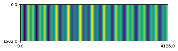
base_path = Path("../tests/data/products").resolve()
test_case: Literal["7_4", "8_2"] = "8_2"
method: Literal["spatial_corr", "spatial_dft", "temporal_corr"] = "spatial_corr"

product_path: Path = base_path / "products" / f"SWASH_{test_case}/testcase_{test_case}.tif"
config_path: Path = base_path / f"reference_results/debug_pointswash_{method}/wave_bathy_inversion_config.yaml"
debug_file: Path = base_path / f"debug_points/debug_points_SWASH_{test_case}.yaml"

# config = read_config(config_path=config_path)

# OR

config = BathyConfig(
    GLOBAL_ESTIMATOR=GlobalEstimatorConfig(
        WAVE_EST_METHOD="SPATIAL_CORRELATION",
        SELECTED_FRAMES=[10, 13],
        DXP=50,
        DYP=500,
        NKEEP=5,
        WINDOW=400,
        SM_LENGTH=100,
        MIN_D=2,
        MIN_T=3,
        MIN_WAVES_LINEARITY=0.01,
    )
)

If you want to change any parameter of the configuration, modify the values of the object config by overriding the values of the attributes.

Example:

config.parameter = "new_value"

bathy_estimator, ortho_bathy_estimator = initialize_sequential_run(
    product_path=product_path,
    config=config,
    delta_time_provider=None,
)

plt_min = bathy_estimator.local_estimator_params['DEBUG']['PLOT_MIN']
plt_max = bathy_estimator.local_estimator_params['DEBUG']['PLOT_MAX']

/home/geoffrey/miniconda3/envs/env_name/lib/python3.12/site-packages/distributed/node.py:187: UserWarning: Port 8787 is already in use.
Perhaps you already have a cluster running?
Hosting the HTTP server on port 44025 instead
  warnings.warn(

estimation_point = Point(451.0, 499.0)

ortho_sequence = build_ortho_sequence(ortho_bathy_estimator, estimation_point)
local_estimator = SpatialCorrelationBathyEstimatorDebug(
    estimation_point,
    ortho_sequence,
    bathy_estimator,
)

if not local_estimator.can_estimate_bathy():
    raise WavesEstimationError("Cannot estimate bathy.")

Preprocess images

Modified attributes: - local_estimator.ortho_sequence.<elements>.pixels

from s2shores.generic_utils.image_filters import desmooth, detrend

def custom_filter(img, param1, param2):
    """My custom filter."""
    return img


if False:
    local_estimator.preprocess_images()
else:
    preprocessing_filters = [(detrend, [])]

    if bathy_estimator.smoothing_requested:
        # FIXME: pixels necessary for smoothing are not taken into account, thus
        # zeros are introduced at the borders of the window.

        preprocessing_filters += [
            (desmooth,
             [bathy_estimator.smoothing_lines_size,
              bathy_estimator.smoothing_columns_size]),
            # Remove tendency possibly introduced by smoothing, specially on the shore line
            (detrend, []),
            # Add your custom filters here
            # Ex: (custom_filter, [param1, param2])
        ]


    for image in local_estimator.ortho_sequence:
        filtered_image = image.apply_filters(preprocessing_filters)
        image.pixels = filtered_image.pixels

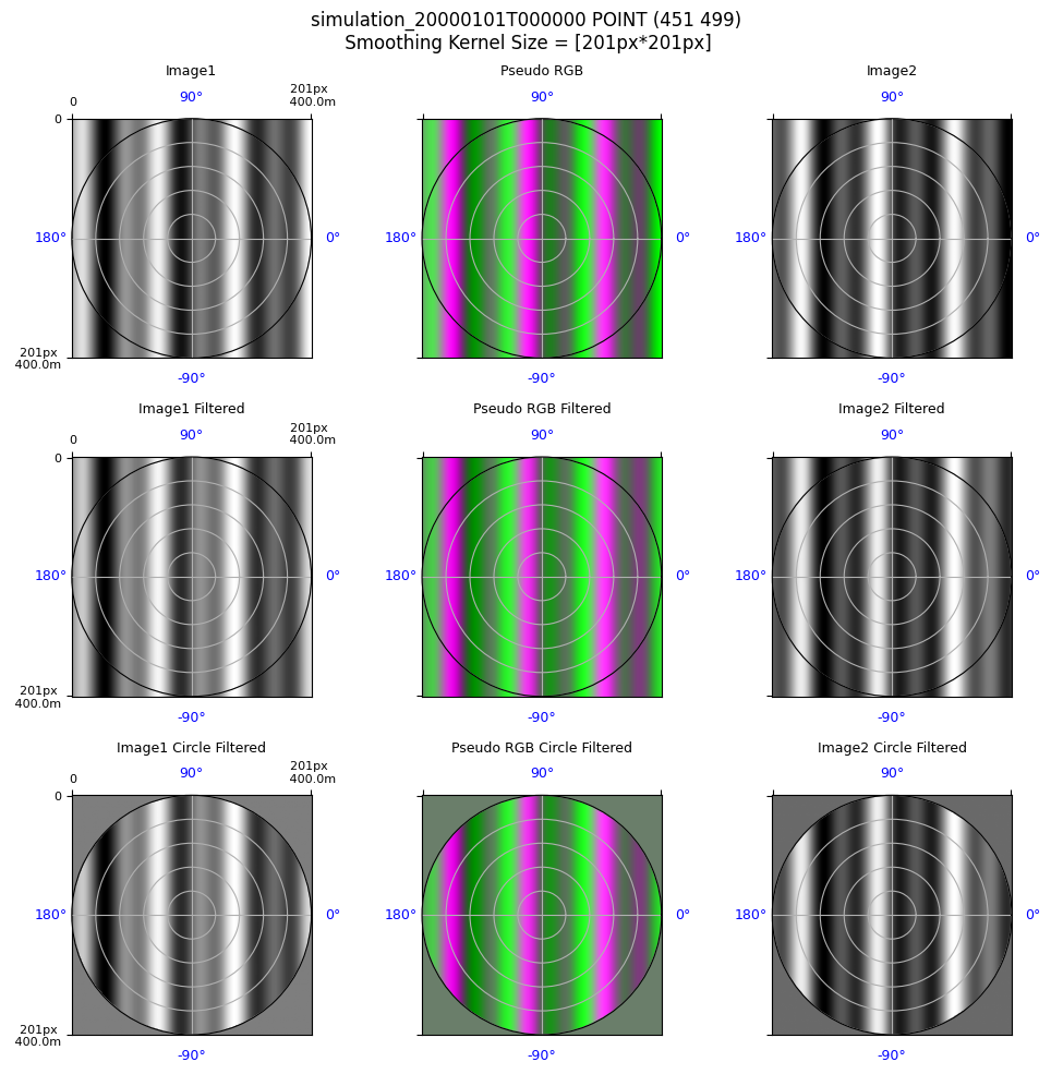
Display processed images

if False:
    build_waves_images_spatial_correl(local_estimator)
else:
    nrows = 3
    ncols = 3
    fig, axs = plt.subplots(nrows=nrows, ncols=ncols, figsize=(10, 10))
    fig.suptitle(get_display_title_with_kernel(local_estimator), fontsize=12)

    first_image = local_estimator.ortho_sequence[0]
    second_image = local_estimator.ortho_sequence[1]

    # First Plot line = Image1 / pseudoRGB / Image2
    plot_waves_row(fig=fig,
                   axs=axs,
                   row_number=0,
                   pixels1=first_image.original_pixels,
                   resolution1=first_image.resolution,
                   pixels2=second_image.original_pixels,
                   resolution2=first_image.resolution,
                   nrows=3,
                   ncols=3)
    # Second Plot line = Image1 Filtered / pseudoRGB Filtered/ Image2 Filtered
    plot_waves_row(fig=fig,
                   axs=axs,
                   row_number=1,
                   pixels1=first_image.pixels,
                   resolution1=first_image.resolution,
                   pixels2=second_image.pixels,
                   resolution2=first_image.resolution,
                   title_suffix=" Filtered",
                   nrows=3,
                   ncols=3)

    # Third Plot line = Image1 Circle Filtered / pseudoRGB Circle Filtered/ Image2 Circle Filtered
    plot_waves_row(fig=fig,
                   axs=axs,
                   row_number=2,
                   pixels1=first_image.pixels * first_image.circle_image,
                   resolution1=first_image.resolution,
                   pixels2=second_image.pixels * second_image.circle_image,
                   resolution2=first_image.resolution,
                   title_suffix=" Circle Filtered",
                   nrows=3,
                   ncols=3)
    plt.tight_layout()

Find direction

New variables: - estimated_direction

if False:
    main_direction = local_estimator.find_direction()
else:
    # Start: WavesRadon(self.ortho_sequence[0], self.selected_directions)
    image = local_estimator.ortho_sequence[0]
    sampling_frequency = 1. / image.resolution
    selected_directions = local_estimator.selected_directions

    pixels = circular_masking(image.pixels.copy())
    radon_transform = symmetric_radon(image=pixels, theta=selected_directions)

    waves_radon = {
        direction: radon_transform[:, idx]
        for idx, direction in enumerate(selected_directions)
    }
    # End: WavesRadon


    # Start: WavesRadon.get_direction_maximum_variance()

    # Start: Sinograms.get_sinograms_variances(selected_directions)
    variances = np.empty(len(selected_directions), dtype=np.float64)
    for result_index, direction in enumerate(selected_directions):
        variances[result_index] = float(np.var(waves_radon[direction]))
    # End: Sinograms.get_sinograms_variances

    index_max_variance = np.argmax(variances)
    main_direction = selected_directions[index_max_variance]
    # End: WavesRadon.get_direction_maximum_variance

main_direction

-180.0

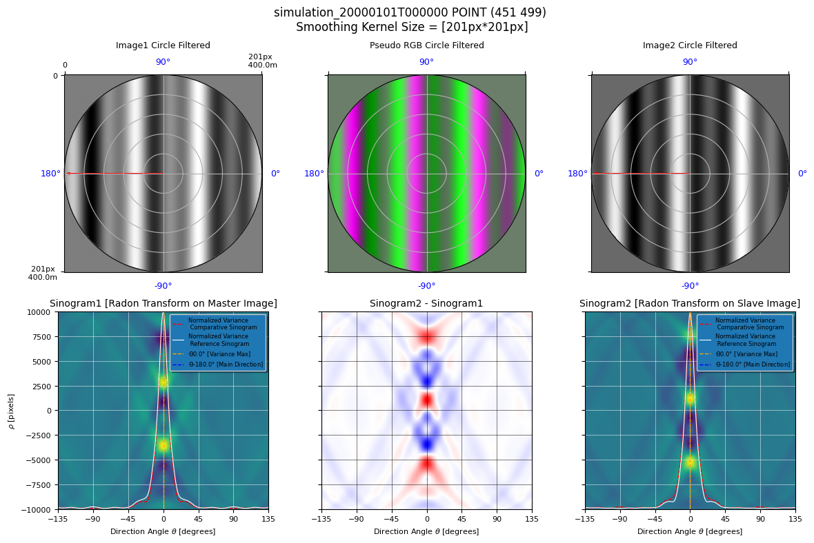
Compute radon transforms

New elements: - local_estimator.randon_transforms

from s2shores.image_processing.waves_radon import linear_directions

# For debugging, all plotted directions need to be computed
min_dir = min(plt_min, min(local_estimator.selected_directions))
max_dir = max(plt_max, max(local_estimator.selected_directions))
selected_directions = linear_directions(angle_min=min_dir, angle_max=max_dir, angles_step=1)

# Reset radon transforms when cell is re-run
local_estimator.radon_transforms = []

if False:
    local_estimator.compute_radon_transforms(main_direction)
else:
    for image in local_estimator.ortho_sequence:
        # Start: WavesRadon(image, np.array([estimated_direction]))
        sampling_frequency = 1. / image.resolution

        pixels = circular_masking(image.pixels.copy())
        radon_transform = symmetric_radon(image=pixels, theta=selected_directions)

        waves_radon = {
            direction: radon_transform[:, idx]
            for idx, direction in enumerate(selected_directions)
        }
        # End: WavesRadon

        # Start: Sinograms.radon_augmentation(self.radon_augmentation_factor)
        radon_augmented = {}
        for direction, values in waves_radon.items():
            current_axis = np.linspace(0, values.size - 1, values.size)
            nb_over_samples = round(((values.size - 1) / local_estimator.radon_augmentation_factor) + 1)
            new_axis = np.linspace(
                start=0,
                stop=values.size - 1,
                num=nb_over_samples,
            )
            interpolating_func = interp1d(current_axis, values, kind='linear', assume_sorted=True)
            radon_augmented[direction] = interpolating_func(new_axis)
        # End: Sinograms.radon_augmentation(self.radon_augmentation_factor)

        local_estimator.radon_transforms.append(radon_augmented)

if False:
    # Use this when computing radon transforms with the standard method
    build_sinograms_spatial_correlation(local_estimator, main_direction)
else:
    nrows = 2
    ncols = 3
    fig, axs = plt.subplots(nrows=nrows, ncols=ncols, figsize=(12, 8))
    fig.suptitle(get_display_title_with_kernel(local_estimator), fontsize=12)
    first_image = local_estimator.ortho_sequence[0]
    second_image = local_estimator.ortho_sequence[1]

    arrows = [(main_direction, np.shape(first_image.original_pixels)[0])]

    # First Plot line = Image1 Circle Filtered / pseudoRGB Circle Filtered/ Image2 Circle Filtered
    plot_waves_row(
        fig=fig,
        axs=axs,
        row_number=0,
        pixels1=first_image.pixels * first_image.circle_image,
        resolution1=first_image.resolution,
        pixels2=second_image.pixels * second_image.circle_image,
        resolution2=first_image.resolution,
        nrows=nrows,
        ncols=ncols,
        title_suffix=" Circle Filtered",
        directions=arrows,
    )

    # Second Plot line = Sinogram1 / Sinogram2-Sinogram1 / Sinogram2
    first_radon_transform = local_estimator.radon_transforms[0]
    second_radon_transform = local_estimator.radon_transforms[1]


    first_iter = next(iter(first_radon_transform.values()))
    nb_samples = first_iter.shape[0]

    sinogram1 = np.empty((nb_samples, len(selected_directions)))
    sinogram2 = np.empty((nb_samples, len(selected_directions)))

    for index, direction in enumerate(selected_directions):
        sinogram1[:, index] = first_radon_transform[direction]
        sinogram2[:, index] = second_radon_transform[direction]

    radon_difference = (
        (sinogram2 / np.abs(sinogram2).max())
        - (sinogram1 / np.abs(sinogram1).max())
    )

    build_sinogram_display(
        axes=axs[1, 0],
        title='Sinogram1 [Radon Transform on Master Image]',
        values1=sinogram1,
        directions=selected_directions,
        values2=sinogram2,
        main_theta=main_direction,
        plt_min=plt_min,
        plt_max=plt_max,
    )
    build_sinogram_difference_display(
        axes=axs[1, 1],
        title='Sinogram2 - Sinogram1',
        values=radon_difference,
        directions=selected_directions,
        plt_min=plt_min,
        plt_max=plt_max,
        cmap='bwr',
    )
    build_sinogram_display(
        axes=axs[1, 2],
        title='Sinogram2 [Radon Transform on Slave Image]',
        values1=sinogram2,
        directions=selected_directions,
        values2=sinogram1,
        main_theta=main_direction,
        plt_min=plt_min,
        plt_max=plt_max,
        ordonate=False,
    )

    plt.tight_layout()

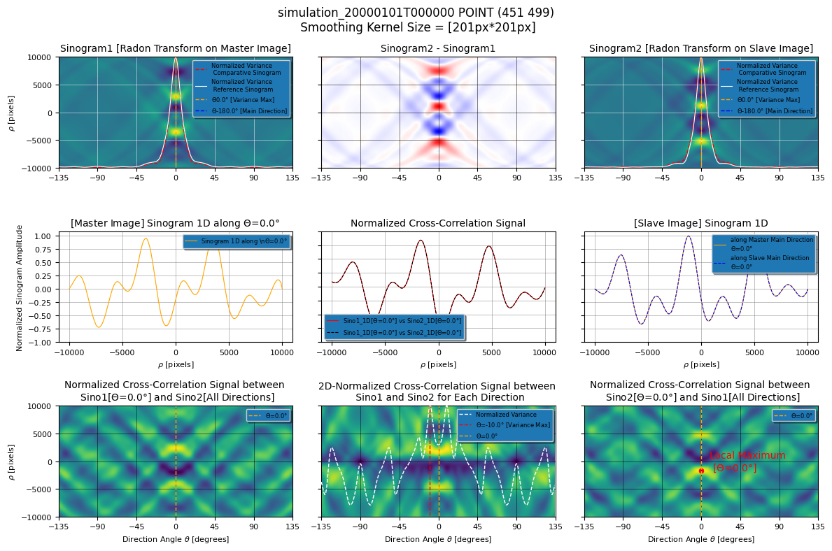
Compute spatial correlation

New elements: - local_estimator.sinograms

New variables: - correlation_signal

local_estimator.sinograms = []

if False:
    correlation_signal = local_estimator.compute_spatial_correlation(main_direction)
else:
    for radon_transform in local_estimator.radon_transforms:
        values = radon_transform[main_direction]
        values *= float(np.var(values))
        local_estimator.sinograms.append(values)
    # TODO: should be independent from 0/1 (for multiple pairs of frames)
    sinogram_1 = local_estimator.sinograms[0]
    sinogram_2 = local_estimator.sinograms[1]
    correl_mode = local_estimator.local_estimator_params['CORRELATION_MODE']
    corr_init = normalized_cross_correlation(sinogram_1, sinogram_2, correl_mode)
    corr_init_ac = normalized_cross_correlation(corr_init, corr_init, correl_mode)
    corr_1 = normalized_cross_correlation(corr_init_ac, sinogram_1, correl_mode)
    corr_2 = normalized_cross_correlation(corr_init_ac, sinogram_2, correl_mode)
    correlation_signal = normalized_cross_correlation(corr_1, corr_2, correl_mode)

correlation_signal

array([0.17217606, 0.17246987, 0.17276372, ..., 0.13137046, 0.13173335,
       0.13209611])

nrows = 3
ncols = 3
fig, axs = plt.subplots(nrows=nrows, ncols=ncols, figsize=(12, 8))
fig.suptitle(get_display_title_with_kernel(local_estimator), fontsize=12)


# First Plot line = Sinogram1 / Sinogram2-Sinogram1 / Sinogram2
radon_difference = (sinogram2 / np.max(np.abs(sinogram2))) - \
    (sinogram1 / np.max(np.abs(sinogram1)))

build_sinogram_display(
    axes=axs[0, 0],
    title='Sinogram1 [Radon Transform on Master Image]',
    values1=sinogram1,
    directions=selected_directions,
    values2=sinogram2,
    plt_min=plt_min,
    plt_max=plt_max,
    main_theta=main_direction,
    abscissa=False,
)
build_sinogram_difference_display(
    axs[0, 1],
    'Sinogram2 - Sinogram1',
    radon_difference,
    selected_directions,
    plt_min,
    plt_max,
    abscissa=False,
    cmap='bwr',
)
build_sinogram_display(
    axes=axs[0, 2],
    title='Sinogram2 [Radon Transform on Slave Image]',
    values1=sinogram2,
    directions=selected_directions,
    values2=sinogram1,
    plt_min=plt_min,
    plt_max=plt_max,
    main_theta=main_direction,
    ordonate=False,
    abscissa=False,
)

# Second Plot line = SINO_1 [1D along estimated direction] / Cross-Correlation Signal /
# SINO_2 [1D along estimated direction resulting from Image1]
# Check if the main direction belongs to the plotting interval [plt_min:plt_max]
if main_direction < plt_min or main_direction > plt_max:
    theta_label = main_direction % (-np.sign(main_direction) * 180.0)
else:
    theta_label = main_direction
title_sino1 = '[Master Image] Sinogram 1D along $\\Theta$={:.1f}° '.format(theta_label)
title_sino2 = '[Slave Image] Sinogram 1D'.format(theta_label)
correl_mode = local_estimator.global_estimator.local_estimator_params['CORRELATION_MODE']

build_sinogram_1D_display_master(
    axs[1, 0],
    title_sino1,
    sinogram1,
    selected_directions,
    main_direction,
    plt_min,
    plt_max,
)
build_sinogram_1D_cross_correlation(
    axs[1, 1],
    'Normalized Cross-Correlation Signal',
    sinogram1,
    selected_directions,
    main_direction,
    sinogram2,
    selected_directions,
    plt_min,
    plt_max,
    correl_mode,
    ordonate=False,
)
build_sinogram_1D_display_slave(
    axs[1, 2],
    title_sino2,
    sinogram2,
    selected_directions,
    main_direction,
    plt_min,
    plt_max,
    ordonate=False,
)

# Third Plot line = Image [2D] Cross correl Sino1[main dir] with Sino2 all directions /
# Image [2D] of Cross correlation 1D between SINO1 & SINO 2 for each direction /
# Image [2D] Cross correl Sino2[main dir] with Sino1 all directions
# Check if the main direction belongs to the plotting interval [plt_min:plt_ramax]

title_cross_correl1 = 'Normalized Cross-Correlation Signal between \n Sino1[$\\Theta$={:.1f}°] and Sino2[All Directions]'.format(
    theta_label)
title_cross_correl2 = 'Normalized Cross-Correlation Signal between \n Sino2[$\\Theta$={:.1f}°] and Sino1[All Directions]'.format(
    0)
title_cross_correl_2D = '2D-Normalized Cross-Correlation Signal between \n Sino1 and Sino2 for Each Direction'

build_sinogram_2D_cross_correlation(
    axs[2, 0],
    title_cross_correl1,
    sinogram1,
    selected_directions,
    main_direction,
    sinogram2,
    plt_min,
    plt_max,
    correl_mode,
    choice='one_dir',
    imgtype='master',
)
build_sinogram_2D_cross_correlation(
    axs[2, 1],
    title_cross_correl_2D,
    sinogram1,
    selected_directions,
    main_direction,
    sinogram2,
    plt_min,
    plt_max,
    correl_mode,
    choice='all_dir',
    imgtype='master',
    ordonate=False,
)
build_sinogram_2D_cross_correlation(
    axs[2, 2],
    title_cross_correl2,
    sinogram2,
    selected_directions,
    main_direction,
    sinogram1,
    plt_min,
    plt_max,
    correl_mode,
    choice='one_dir',
    imgtype='slave',
    ordonate=False,
)

plt.tight_layout()

Compute wavelength

Modified attributes: - None

New variables: - wavelength

if False:
    wavelength = local_estimator.compute_wavelength(correlation_signal)
else:
    min_wavelength = wavelength_offshore(
        local_estimator.global_estimator.waves_period_min,
        local_estimator.gravity,
    )
    min_period_unitless = int(min_wavelength / local_estimator.augmented_resolution)
    try:
        # Depending on the input signal, the resulting period is either in space or time (in this case, space)
        period, _ = find_period_from_zeros(correlation_signal, min_period_unitless)
        wavelength = period * local_estimator.augmented_resolution
    except ValueError as excp:
        raise NotExploitableSinogram('Wave length can not be computed from sinogram') from excp

wavelength

134.68150021791905

Compute delta position

Modified attributes: - None

New variables: - delta_position

if False:
    delta_position = local_estimator.compute_delta_position(correlation_signal, wavelength)
else:
    peaks_pos, _ = find_peaks(correlation_signal)
    if peaks_pos.size == 0:
        raise WavesEstimationError('Unable to find any directional peak')
    argmax_ac = len(correlation_signal) // 2
    relative_distance = (peaks_pos - argmax_ac) * local_estimator.augmented_resolution

    celerity_offshore_max = celerity_offshore(
        local_estimator.global_estimator.waves_period_max,
        local_estimator.gravity,
    )
    spatial_shift_offshore_max = celerity_offshore_max * local_estimator.propagation_duration
    spatial_shift_min = min(-spatial_shift_offshore_max, spatial_shift_offshore_max)
    spatial_shift_max = -spatial_shift_min

    stroboscopic_factor_offshore = local_estimator.propagation_duration / period_offshore(
        1 / wavelength, local_estimator.gravity)

    if abs(stroboscopic_factor_offshore) >= 1:
        # unused for s2
        print('test stroboscopie vrai')
        spatial_shift_offshore_max = (
            local_estimator.local_estimator_params['PEAK_POSITION_MAX_FACTOR']
            * stroboscopic_factor_offshore
            * wavelength
        )

    pt_in_range = peaks_pos[np.where(
        (relative_distance >= spatial_shift_min)
        & (relative_distance < spatial_shift_max)
    )]
    if pt_in_range.size == 0:
        raise WavesEstimationError('Unable to find any directional peak')
    argmax = pt_in_range[correlation_signal[pt_in_range].argmax()]
    delta_position = (argmax - argmax_ac) * local_estimator.augmented_resolution

delta_position

-38.800000000000004

Save wave field estimation

New elements: - local_estimator.bathymetry_estimations

if False:
    local_estimator.save_wave_field_estimation(main_direction, wavelength, delta_position)
else:
    bathymetry_estimation = local_estimator.create_bathymetry_estimation(main_direction, wavelength)
    bathymetry_estimation.delta_position = delta_position
    local_estimator.bathymetry_estimations.append(bathymetry_estimation)

print(f"Physical: {local_estimator.bathymetry_estimations[0].is_physical()}")
print(local_estimator.bathymetry_estimations[0])

Physical: True
Geometry:   direction: 0.0° wavelength: 134.68 (m) wavenumber: 0.007425 (m-1)
Dynamics:   period: 10.41 (s)  celerity: 12.93 (m/s)
Wave Field Estimation:
  delta time: 3.000 (s) stroboscopic factor: 0.288 (unitless)
  delta position: 38.80 (m)  delta phase:  1.81 (rd)
Bathymetry inversion: depth: 23.43 (m)  gamma: 0.798  offshore period:  9.30 (s)  shallow water period: 30.45 (s)  relative period:  0.89  relative wavelength:  1.25  gravity: 9.780 (s)
Bathymetry Estimation:  stroboscopic factor low depth: 0.099  stroboscopic factor offshore: 0.323